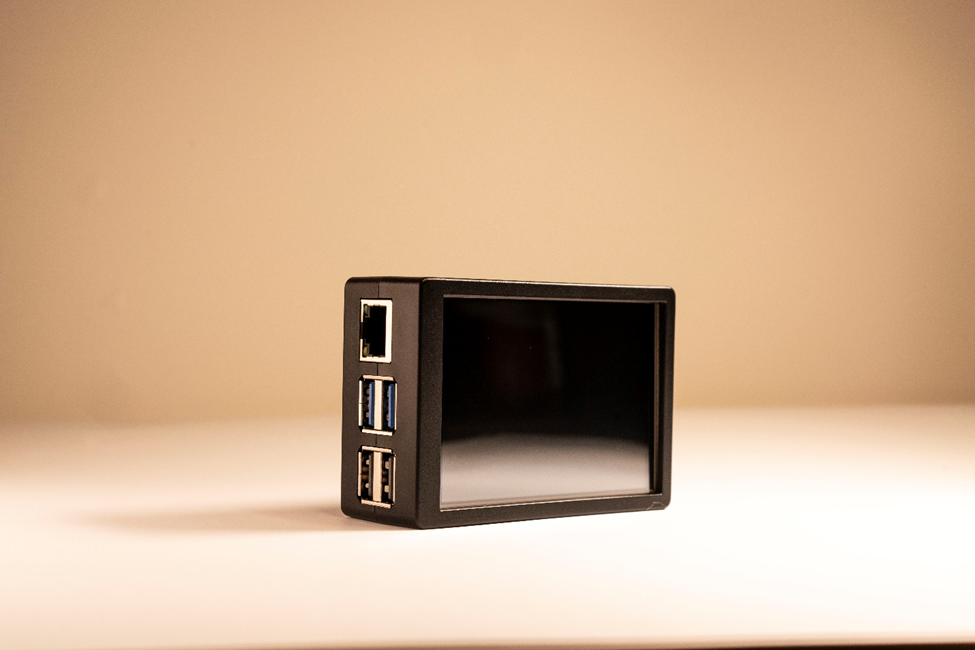
Table of Contents:
– Hardware
– Software
– System Functionality
– GUI Guide/Images
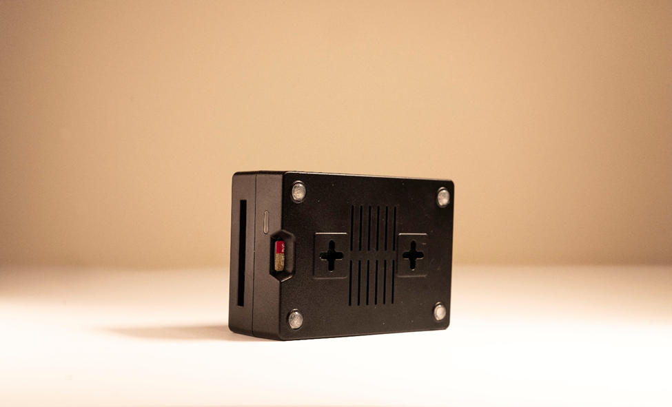
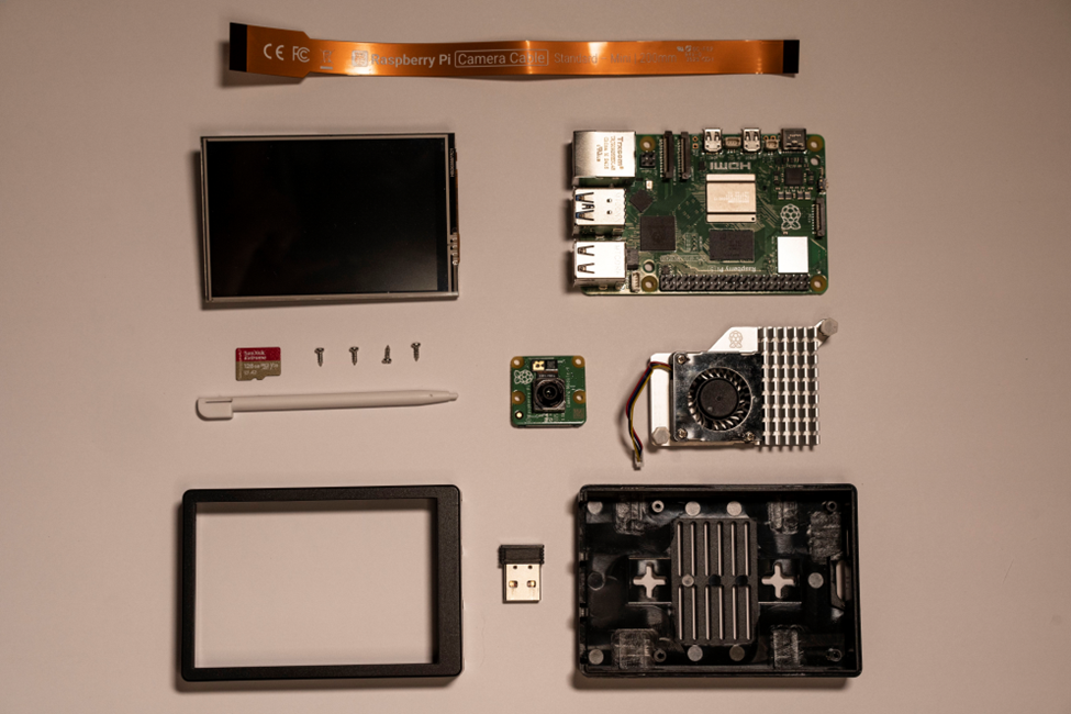
Hardware:
- Raspberry Pi 5 (~189 USD):
– 64-bit quad-core Cortex-A76 processor
– 8GB LPDDR4X SDRAM
– 802.11b/g/n/ac wireless
– Bluetooth 5.0
– 5V/5A USB-C power supply - Raspberry Pi Active Cooler (~11 USD):
– Single-piece anodized aluminum heatsink
– Heatsink-mounted temperature-controlled fan
– Thermal pads for heat transfer - GeekPi Display (~29 USD):
– 3.5 inch LED Screen
– Resolution: 480×320
– MHS Resistive Touch
– ABS Case
– Driver location: wiki.52pi.com/index.php?title=KZ-0060 - Raspberry Pi Camera Module 3 (~49 USD):
– Back-illuminated, stacked CMOS 12-megapixel Sony IMX708 image sensor
– Phase Detection Autofocus (PDAF) for rapid autofocus
– HDR mode (up to 3 megapixel output)
– Resolution: 11.9 megapixels
– Sensor size: 7.4mm sensor diagonal
– Diagonal field of view: 75 degrees - Geekworm Pi5 Battery Pack (~43 USD):
– X1200 5V UPS HAT Shield for Raspberry Pi 5
– Max 5.1V 5A Output | Auto Power On
– Safe Shutdown|Power Loss Detection Function
– Battery 18650 flat-top 3.7 2200mAh Li-ion(x2)
Software:
- Operating System:
– Raspberry Pi OS (64-bit)
– Debian Bookworm base
– Optimized for ARMv8-A architecture - Core Interface:
– Custom Python-based GUI
– Tkinter Toolkit for touch-optimization
– Multi-threaded loop for real-time signal monitoring - Networking Tools:
– Linux Wireless Tools (iwconfig)
– Subprocess interface for kernel-level data extraction
– SSID and dBm signal strength parsing logic - Data Visualization & Processing:
– Inverse Distance Weighting (IDW) interpolation algorithm
– PIL (Pillow) for dynamic image and thumbnail rendering
– JSON-based session storage for survey portability
– Ghostscript/PostScript for high-resolution vector map exports - Camera Integration:
– Picamera2 Python library
– Libcamera backend for hardware-accelerated image processing
– Phase Detection Autofocus (PDAF) control logic
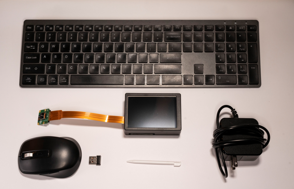
System Functionality:
- Real-Time Analytics:
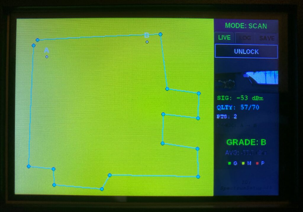
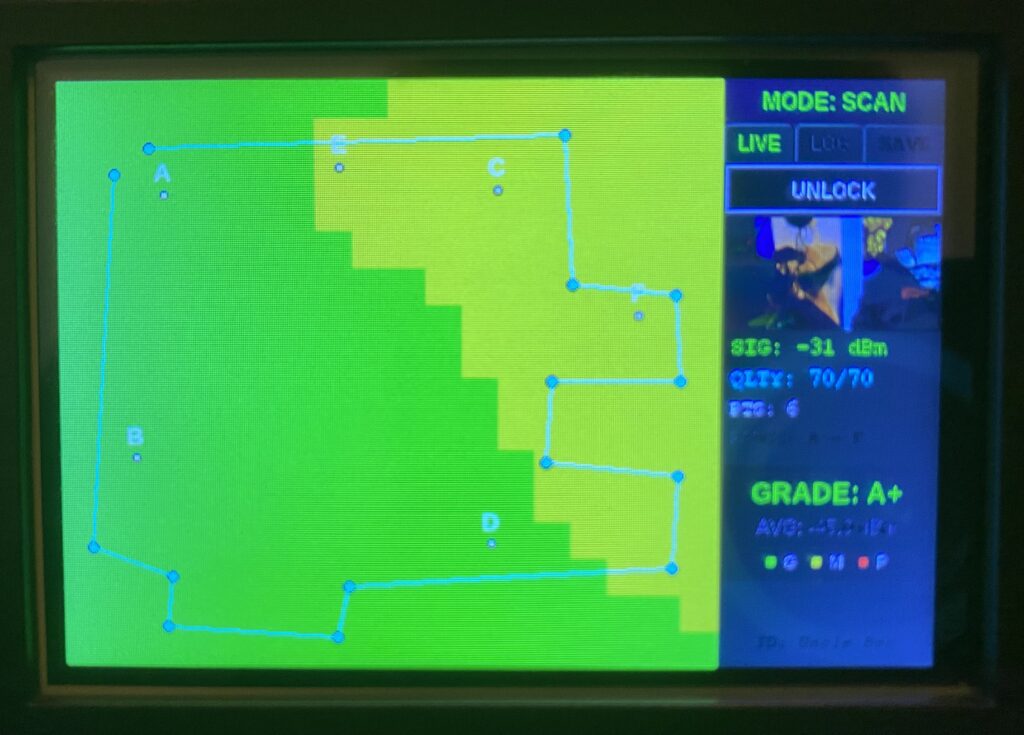
– Dynamic Heatmapping: Generates a color-coded coverage overlay (480×320 resolution) based on spatial signal data.
– Signal Grading: Automated “Grade” calculation (A+ through F) based on office-standard signal thresholds.
– Visual Evidence: Simultaneous 12MP photo capture at each data point to document physical obstructions (walls, metal cabinets, etc.). - User Experience:
– Dual-Mode Workflow: Toggle between ‘Draw Mode’ for architectural layout and ‘Scan Mode’ for data collection.
– Live Telemetry: Real-time dashboard showing current SSID, Link Quality, and dBm levels.
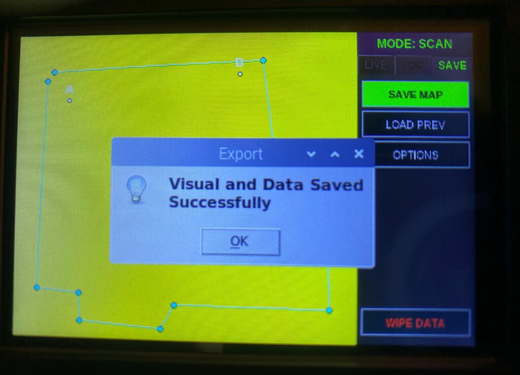
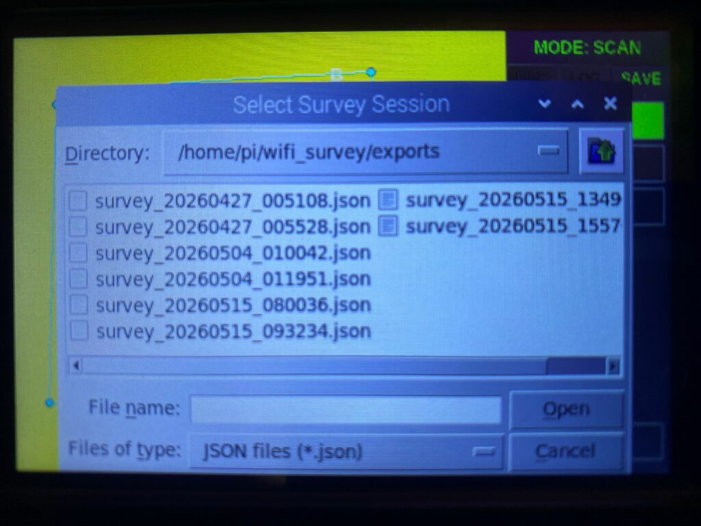
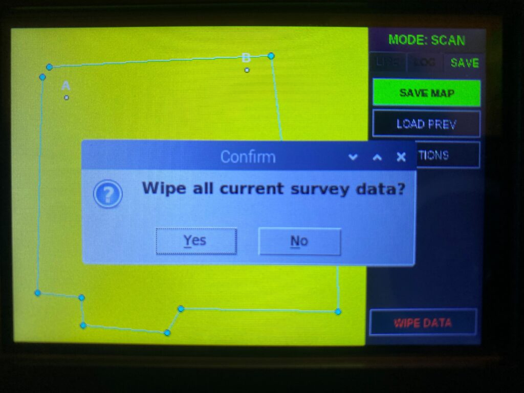
– Session Management: Ability to wipe data, load previous surveys, and export finalized maps for site reports.
GUI Guide/Images
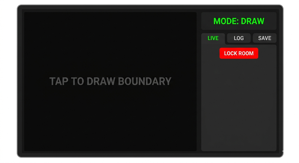
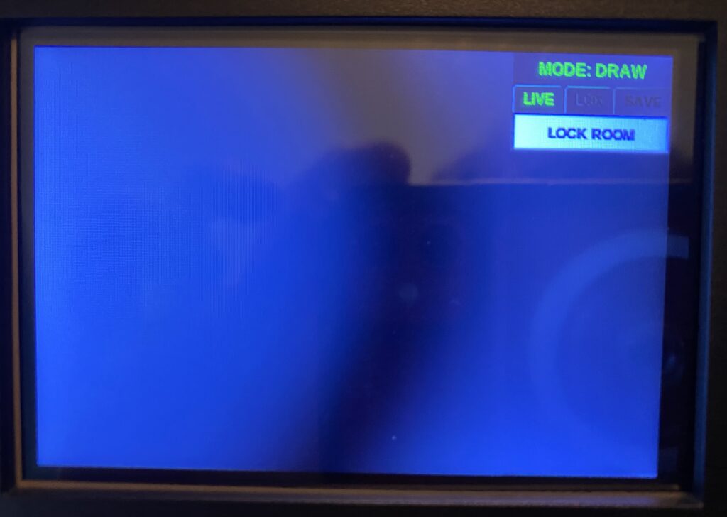
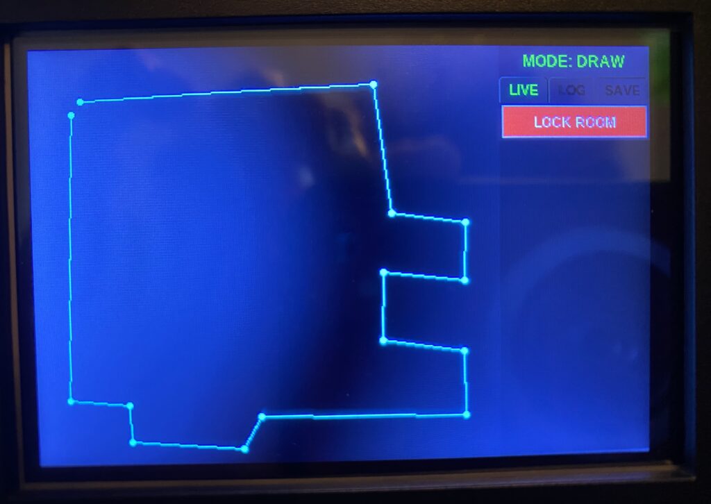
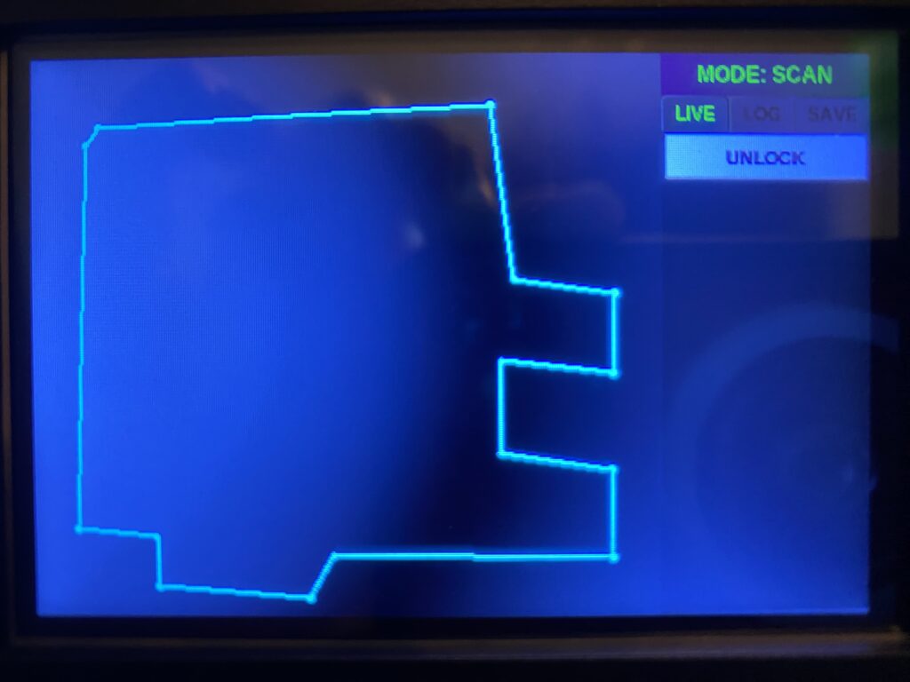
1. Main Interface – “MODE: DRAW”
This image shows the core layout of the application upon startup. The left side features the dark Map Canvas, which displays initial instructions (“TAP TO DRAW”) against an nearly black background.
The right side features the Control Panel, separated into distinct regions. A prominent header strip across the top reads “MODE: DRAW” in bright green text against a dark gray block. Below the header are the three navigation tabs: LIVE, LOG, and SAVE, with the ‘LIVE’ tab currently selected and active.
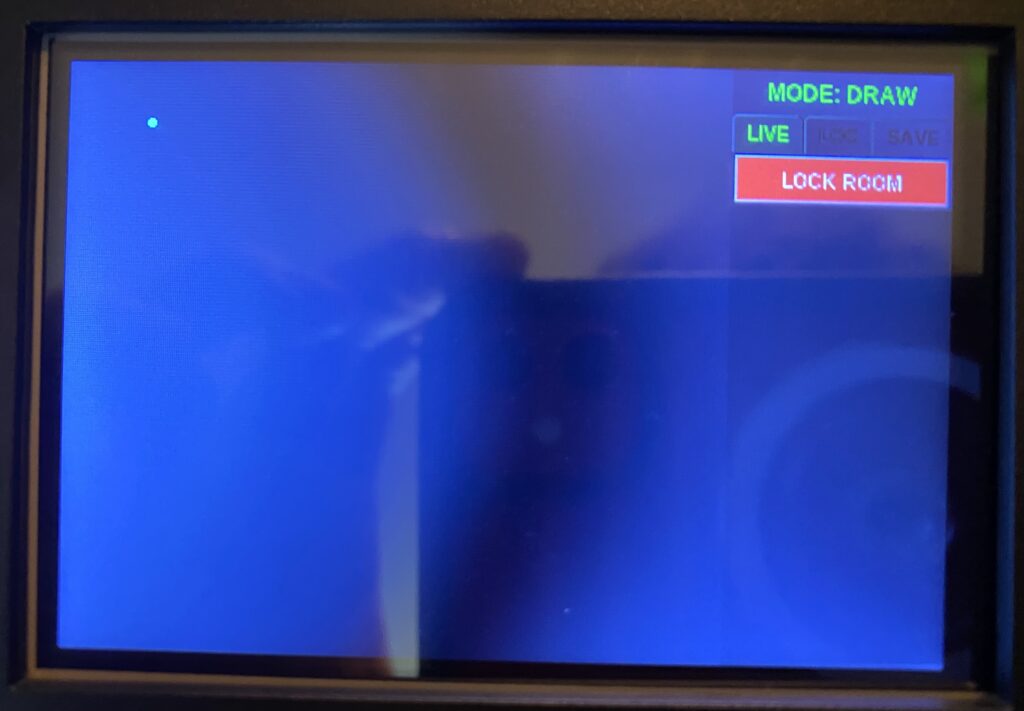
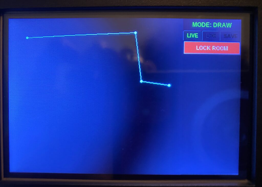
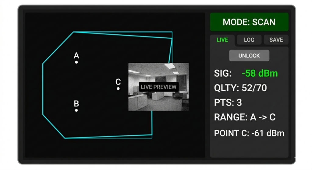
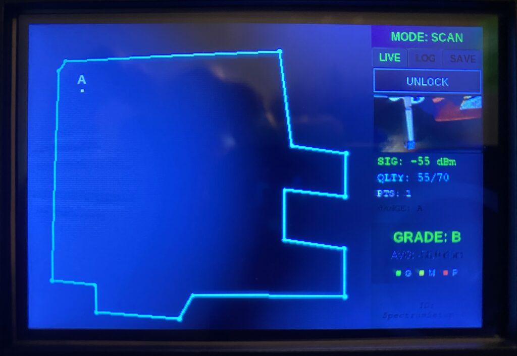
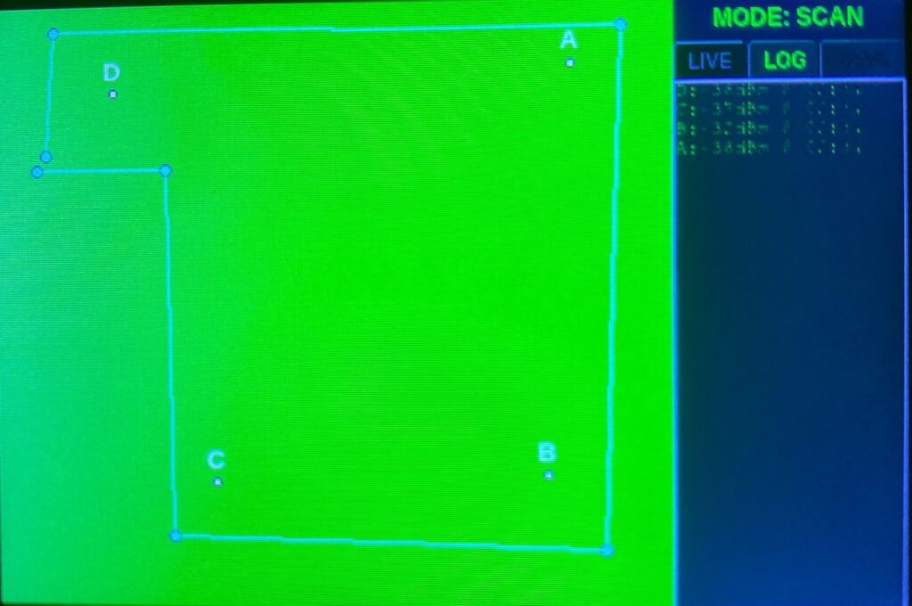
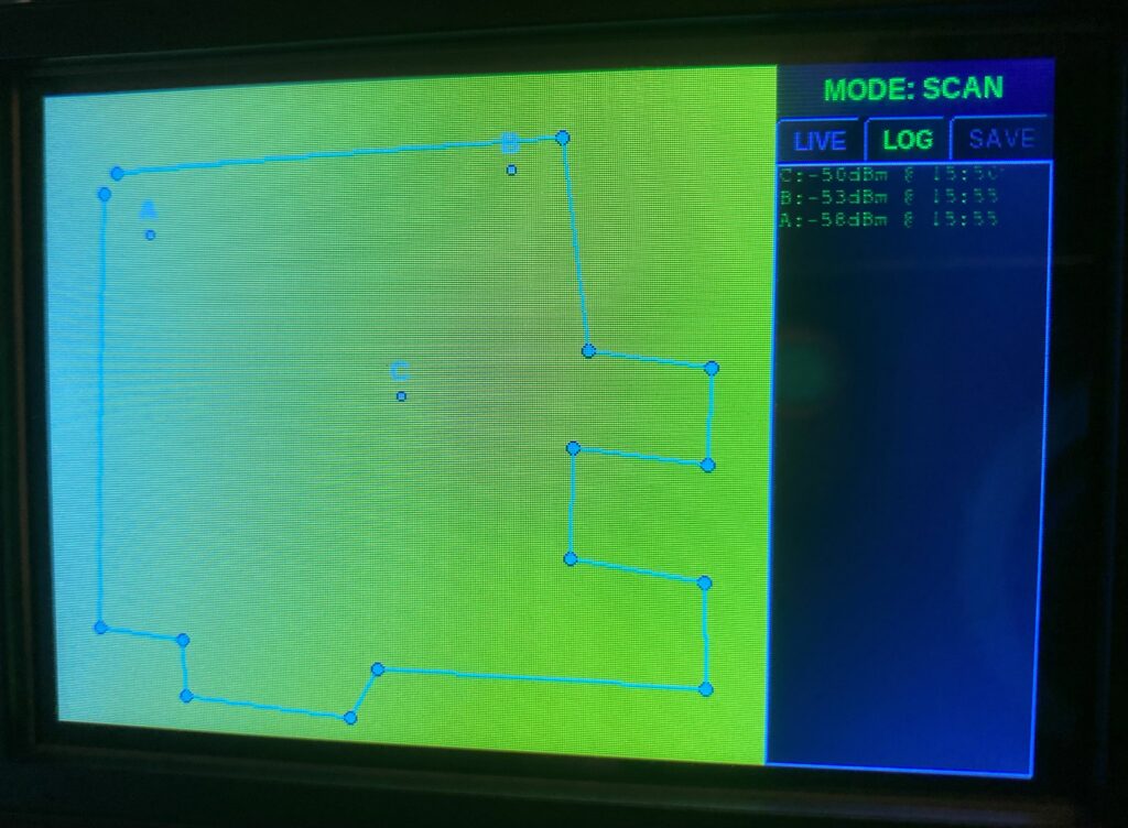
2. Active Survey – “MODE: SCAN”
This rendering simulates an active survey. The application is now in “MODE: SCAN” . A bright cyan room perimeter has been drawn. Within this boundary, three WiFi measurement points are visible: ‘A’, ‘B’, and ‘C’, each marked with a white dot and label.
3. Options Configuration Window
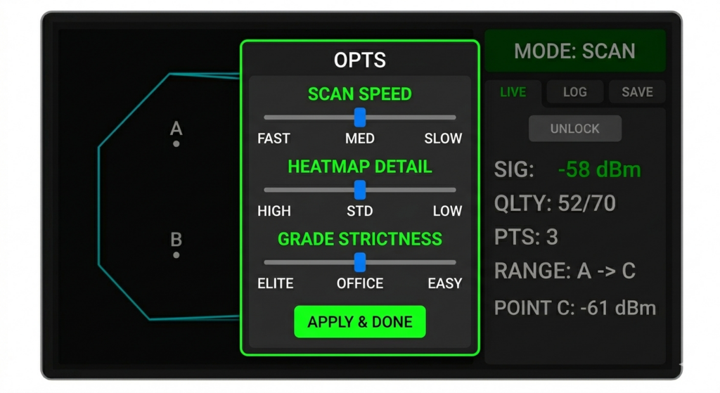
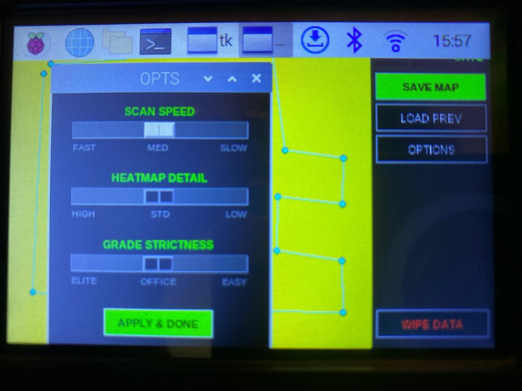
This rendering highlights the tk.Scale sliders defined in your show_options method. The main application is slightly dimmed in the background while a focused “OPTS” configuration popup window takes priority.
The popup uses a dark gray scheme with bright green titles. Three horizontal slide bars are present for “SCAN SPEED”, “HEATMAP DETAIL”, and “GRADE STRICTNESS”. Each slider shows its minimalistic descriptions (e.g., “FAST”, “MED”, “SLOW”) below the bar, clearly indicating the three gradual modes or presets available for that setting, allowing the user to configure the survey performance.
4. Heatmap Generation
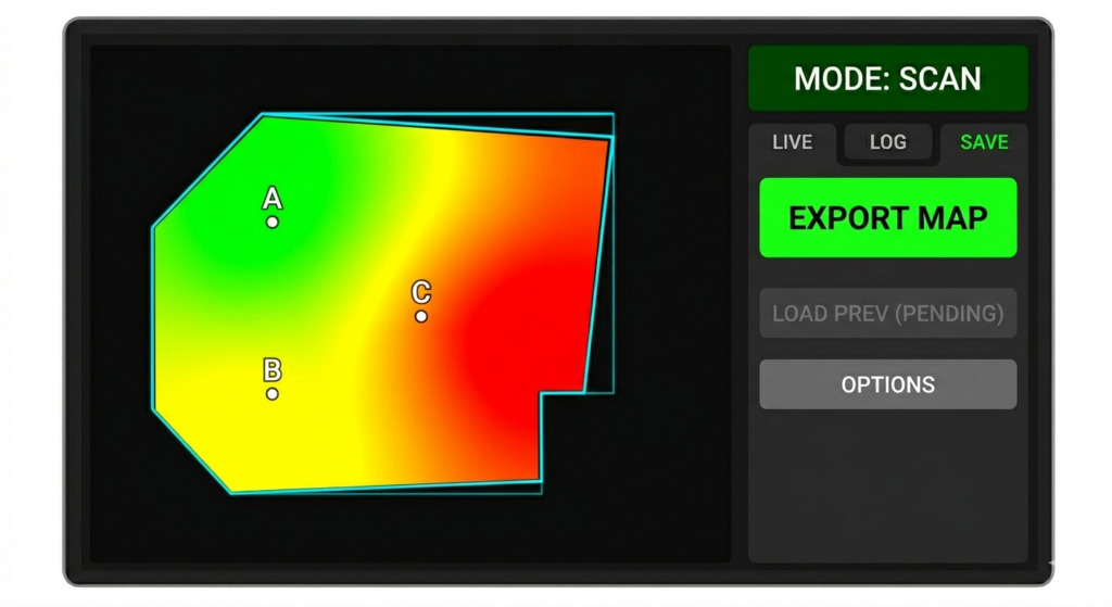
This visualization demonstrates the core function of the application: the generated WiFi heatmap. Following the survey shown in Image 2, the main canvas has now rendered a smooth color gradient across the room floor plan.
The gradient uses green for good signal, yellow for medium, and red for poor. The ‘A’ area shows a strong green signal, while ‘C’ shows a red dead zone. The original point markers (‘A’, ‘B’, ‘C’) are still superimposed on the color map. The right panel is switched to the SAVE tab, where the bright green “EXPORT MAP” button is active, alongside the “LOAD PREV” feature and “OPTIONS”.
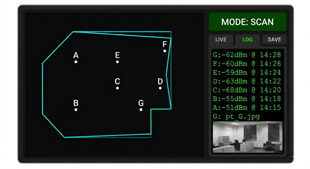
5: Logs
In this visualization, the application remains in “MODE: SCAN” within the drawn perimeter. The right-hand control panel is switched to the LOG tab.
The panel displays a simple, deep black terminal feed. A list of recent WiFi measurements (Points A through G) is printed in monospaced “Courier” font.
Leave a Reply